5. Full Operation of the Tool Bar Tools#
5.1. Results#
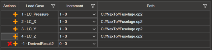
The results bar displays all tools related to visualizing the model’s results:
Load Case: This tool displays all load cases associated with the model, allowing you to select the specific load case you wish to analyze.

Increments: This feature shows the different increment types available within the model, enabling you to choose the type of increment for detailed examination.

Results: Here, you can see the various types of results that the model can generate. Select the desired result type to work with for your analysis.

5.2. Plot Contour#
The “Plot Contour” Tool Bar shows all the tools related to model drawing.
5.2.1. Components#
The components of the model are displayed. It allows to indicate the component on the basis of which the model will be plotted.

5.2.2. Sections#
The sections of the model are displayed. Allows to indicate the section with which the model will be plotted.

5.2.3. Plot contour results#
 Clicking on this icon plots the model based on the load case, increments, results, component and sections indicated.
5.2.4. Plot Vector Results#
 Click this icon to display results in vector mode. Depending on the value and setting the arrows are larger or smaller and have a different color (only for vector results).
5.2.5. Plot Tensor Results#
 Click this icon to display results in tensor mode. Only the tensor results can be painted in this way as stresses.
5.2.6. Clear plot contour results#
 Clicking on this icon clears the plotting of the results that had been plotted.
5.2.7. Plot Contour Options#
Clicking on the gear icon opens a new window that allows you to edit options for specific results.

In the “Elements Domain” section, you select the domain where the results are displayed, with three available options:
All: Displays results for the entire model.
Visualized: Displays results for the parts that are currently visible on the screen.
Selected: Displays results for the specifically selected elements or parts.
Here are three options:
Contour: Settings tab for plot contour.
Vector: Settings tab for plot vector.
Tensor: Settings tab for plot Tensor.
The “At grid position” option displays the results at the node positions, which is activated by checking the respective checkbox.

Within the “Contour” option, various settings can be adjusted such as:
“Averages”
For sections: Allows calculating the average for each section.
For positions: This feature is particularly useful for Abaqus, where certain results might be required at integration points. For example, a QUAD element can have four integration points, and it might be relevant to decide whether the maximum, minimum, or average of the four values is desired.

The “Coordinate System” option allows you to switch the results to a different coordinate system from the element system, which is the default system for results in a binary results file.

Within the “Vector” option, various settings can be adjusted such as:

Is Rotation: This option is selected when you want to represent rotations instead of displacements. Normally, vector results have X, Y, and Z components, but you can also represent rotation in X, Y, and Z.
Color by Value: This option indicates that you want to color the arrows based on their scalar value (similar to how cells are colored in a normal contour plot, but instead of coloring the model, the vectors are painted) rather than using the user-configured color for that component.
Show Text: This option indicates whether you want to display the vector value in a label.

When plotting results in vector or tensor mode, the components selected by the user are not used.

Instead, the configuration of the component is done within this window. To paint vectors, you can paint the X vector, the Y vector, the Z vector, or the resultant by combining them as the sum of the selected components (which would be the magnitude). If you want these values to be Rx, Ry, etc., this is achieved by selecting the previous option “Is Rotation.”

Scaling by: Configures the criterion by which the vector is scaled.
Auto: the application chooses it (by default, it is usually based on the scalar value of the vector).
By Value: scaled according to the value of the vector. Uniform: all vectors are the same size.
Factor: used to change the size factor of the vectors.

Tip: Select the shape of the vector head, either an arrow or none.
Origin: Select where the vector starts when rendered.
Resolution: Configure the level of detail of the vector.
Set Min: Configure the minimum value from which vectors are plotted; any value below this will not create a vector.
Set Max: Configure the maximum value; any value below this scalar will create a vector, if above, it will not. Coord system functions the same as in plot contour.
Within the “Tensor” option, various settings can be adjusted such as:

Color by Value: Colors the tensor based on its value instead of the user-configured color.
Normal Text: Displays labels for the axial or tensor values.
Shear Text: Displays labels for the shear values of the tensor.

Configure which tensor values you want to see and what color you want for each axis or shear.

Scaling by: Configures the criterion by which the tensor is scaled.
Auto: the application chooses it (by default, it is usually based on the scalar value of the tensor).
By Value: scaled according to the value of the vector. Uniform: all tensors are the same size.
Factor: used to change the size factor of the tensors.

Tip: Select the shape of the tensor head, either an arrow or none.
Origin: Select where the tensor starts when rendered.
Resolution: Configure the level of detail of the tensor.
Set Min: Configure the minimum value from which tensors are plotted; any value below this will not create a tensor.
Set Max: Configure the maximum value; any value below this scalar will create a tensor, if above, it will not. Coord system functions the same as in plot contour.
This option is useful when loading a model in frequency response analysis, as it allows you to choose between two representations for “plotting results in complex” numbers: Polar and Cartesian.
To select the desired option, use the Toggle Button.
Polar: Displays the magnitude or phase of the result, depending on the selection made in the component Combo Box.
Cartesian: Displays the real or imaginary part of the result, depending on the selection made in the component Combo Box.

5.2.8. Scalar Bar Options#

This tool facilitates defining the options for the legend. By clicking on the corresponding icon, a new window opens where you can edit various settings.
You can adjust the position of the legend (to the right or left) and customize the font size and style used in the legend information.

Regarding the color options, you can specify:
The number of colors we want the legend to have.
Customize colors by simply clicking on the desired color and selecting the preferred Pantone shade.
Choose the color of the text, the background of the text box, and the border of the text box.

Additionally, you can modify display data, such as font size and style, the number of digits for each value, and numeric format. We can also set the maximum and minimum range of values.
Another option is to invert the legend colors.

The new legend configuration can be saved to a file for future use. To do this, simply click “Export,” select the desired location and name for the *.xml file. If you want to reuse this configuration in the future, you can import the *.xml file by selecting the “Import” option. If you want to restore the original configuration, you can click “ Defaults.”

5.3. Auxiliary Tools#
The “Report Settings” toolbar offers two key features:
5.3.1. Create Derived Results#
 To create generate derived results, click on the “Derived results” icon on toolbar.
This action opens a new window where you can create results based on combinations of different load cases or components using common functions.
5.3.1.1. Derived Load cases based on a function#

This feature enables the creation of a new load case derived from existing ones. Start by naming the new load case.

Select the original load cases you want to combine by clicking the orange plus icon.

Use the table at the bottom to enter and combine expressions. Detailed guidance on defining these expressions is available in 9.1. Reserved words and arithmetic expressions of the derived results.

Once your expression is set, click the green plus icon to finalize the new load case, which will be listed as a negative integer to differentiate it from original load cases.


The newly derived load case also appears in the table with the original load cases.

5.3.1.2. Derived load cases based on an envelope#

This tool creates a new load case from existing ones by calculating the maximum, minimum, extreme values, or the range. Start by naming the new load case.

Select the load cases, increments, and the path. You can choose to apply this to all or select specific ones.

Specify the criterion (Max/Min/ExtremMin/ExtremMax/Range) to apply to the contour values across the selected load cases.

Activate the checkbox if you want all increments within the load cases to be considered, which is useful for comprehensive analysis across multiple increments.

Clicking on the green plus icon will create a new derived load case based on an envelope.

This load case becomes one of the load cases available to the user to plot the results.
Derived load cases are always negative integers, which is what differentiates them from an original load case.

The newly derived load case also appears in the table with the original load cases.
When you select the newly created load case, you choose what you want to see of the envelope: the type of result, the component of that result, etc.
For example, in the newly created component you have chosen the maximum value criterion and, for example, you choose to plot STRESSES, in the VON_MISES component and in the NONE section. When plotting on the screen, the highest value of VON_MISES STRESSES is displayed in each of the displayed elements and occurs among all load cases that had been selected.
After having created the new load case, a new section called “Envelope” appears in the toolbar.
In this section you can select different options that allow you to decide what you want to plot.

ByContour: This is the default option. This option will get the contour, i.e., if you plot DISPLACEMENTS or STRESSES it will get the maximum in that element, in the selected component and for that load case list.
ByLoadCaseID: Plots that the value to assign to the element is the ID of the load case that produces that maximum displacement or stress.
ByIncrement: What is plotted, i.e., that the value to assign to the element is the ID of the increment, which produces the maximum, minimum, etc., contour in that element.
5.3.1.3. Results derived from the Component#

This option allows for the creation of new components by combining existing ones within a result type.
Name the new component.

Select the result type it relates to.

Choose components to combine and enter the expressions for combining them as previously described.

The table at the bottom is where the regular expressions are shown. They can be combined and operated on. The question is to define the expression. In section 9.1. Reserved words and arithmetic expressions of the derived results. , explains how to do it correctly.

The new component will appear under the selected result type when accessing any load case, including derived ones.
o For example: It has been created in *DISPLACEMENTS* and called *"Magnitude_Displacements"*.
Thus within “DISPLACEMENTS” which is the result type, a new component called “Displacements_Magnitude” will appear.
Thus, when accessing any load case, including derived load cases, the new component created will appear under “DISPLACEMENTS”.

The newly derived load case also appears in the table with the original Components.

5.3.1.4. How edit and delete Derived Results#
Derived results, whether they are load cases or components, can be edited or deleted as needed.
To edit, select the desired derived result from the list, make the changes, and save by clicking the floppy disk icon.
To delete a derived result, click on the X icon.

5.3.2. Report Settings#

The “Report Settings” tool allows you to select a series of results and export them to Excel.
To begin, click on the following icon to choose where to save the .csv file and provide a name for it. The path where the file will be saved is recorded in the “Path” section.

5.3.2.1. Steps to Create the Report#
Select Elements/Nodes
Choose the Elements/Nodes from the model for which you want to extract results.
After making your selection, click on the green plus icon.
The number of selected Elements/Nodes will be displayed.
You can hide or show the selected Elements/Nodes by toggling the eye icon.

Configure Load Cases and Increments
The table will show the load cases, increments, and the file path.
Select the load cases and increments you wish to export.
To select all increments for the chosen load cases, use the checkbox at the bottom right of the table.

Select Result Types
Choose the type of results to export.
In the table below, select the components and sections you want to include in the export.

Organize the .csv File
Choose how to organize the .csv file:
By Load Case: Displays the selected results for each load case.
By Elements/Nodes: Displays the selected results for each element/node.
If you select the “Output with only envelope” option, only the envelope results of the model will be included.

Generate the Report
After selecting all necessary fields, click on “Generate report” to save the .csv file with the chosen name and path.

5.3.2.2. Contour Settings#
Clicking on this icon opens a new window to edit contour settings.

At Grid Position:
 Displays results at node positions, activated by checking the corresponding box.
Contour Settings:
Averages:
For Sections: Calculates the average for each section.
For Positions: Useful for Abaqus, where certain results at integration points might be needed. For instance, a QUAD element might have four integration points, and you can decide whether to take the maximum, minimum, or average of these values.
5.4. Animation Setting#

The animation tool allows you to animate the specified load cases in the model and their increments. There are two types of animations available:

Transient: Animates all increments of a load case.
Linear: Animates from the initial state (0) to the final state of the selected increment, with the steps defined in the “Steps” section.
5.4.1. Animation Controls#
5.4.1.1. Timeline#
The animation timeline is located at the bottom of the animation bar.

5.4.1.2. Main Controls#

In the center of the animation bar, you will find the following buttons:
 Start Animation: Begins the animation.
 Pause Animation: Pauses the animation.
 Previous Increment: Moves to the previous increment.
 Next Increment: Advances to the next increment.
 Start of Animation: Returns to the beginning of the animation.
 End of Animation: Moves to the end of the animation.
5.4.1.3. Editing Options (Right Side of the Bar)#

Animation Start: Selects the increment where the animation starts.
Animation End: Selects the increment where the animation ends.
Framerate: Controls the speed of the animation in frames per second. A value of 1 will advance one increment per second.
Increment By: Specifies the increment between animation steps. For example, a value of 2 will advance in steps of 2.
Interpolations: Estimates the data between increments. If there are 7 increments and 2 interpolations are specified, there will be 21 increments in total.
Scale: Defines the deformation scale of the model. Enter the desired deformation value.
5.4.1.4. Animation Controls (Left Side of the Bar)#

Loop: If checked, the animation restarts from the beginning once it finishes.
Bounce: If checked, the animation reverses direction once it reaches the end.
Note: Checking one of these options will automatically uncheck the other.
Forwards/Backwards: Determines the direction of the animation. “Forwards” moves the animation forward, “Backwards” moves it backward.
Update Legend: If checked, the legend shows the maximum and minimum values of each frame during the animation.
Save: Saves the animation as a video in *.avi format.
5.4.1.5. Additional Notes#
Unlike the Transient option, the Linear option does not include the start and end animation buttons, as they are not relevant in this context. All other controls are the same as in the Transient option.
To apply interpolations, steps, and other settings, the animation must be paused.
While the animation is active, the general toolbar of NaxToView is locked.
5.5. Free Bodies Settings#

The Free Bodies tool, is designed for creating sections within a model’s structure to measure forces passing through. This tool is applicable only in models that include GP Forces.
This tool is segmented into three parts: the first part configures the sections, the second selects load cases and increments for calculating Free Bodies, and the third displays the calculated Free Bodies results.
5.5.1. Configure the Free Bodies sections.#
 To create sections, click the icon in the top-right corner to add multiple sections.

To delete a section, simply click on the icon on the left.

In the first column you can change the name by double clicking on the box.
For the subsequent sections, load the necessary elements, nodes, coordinate system, origin, and parts required to configure the section. Detailed explanations for each section follow
 To add the elements, select them within the model. Once selected, click on the plus icon, and the elements of that section will automatically load.

Clicking on the eye icon, which appears uncrossed, enables you to view the elements marked within the section. This visibility makes it easier to select nodes associated with those elements
 To add nodes, you have to do the same, select the nodes and click on the plus button to load them.
 As for the coordinate system there are 3 options:
The global one is used by default.
Select a coordinate system from the model
Create a new coordinate system. Section 6.1.2.1. Create a new coordinate system explains how to do this.
Select one, the selected coordinate appears in pink. Then click on the plus icon to load the coordinate system selected in the section.
 The next step to configure the section is the point. There are 3 configuration options:
By default, the centroid is checked, the centroid is the center of the section nodes.
Select the X, Y and Z coordinates.
If you select, for example, a node and press the plus button automatically load the coordinates of that node X, Y, and Z, therefore, the origin of the Free Bodies calculation would be that point.
 The last column to configure the section is the part. It is important that both the elements and the nodes of the section are of the same part.
To finish explaining this first part, the following icon remains to be explained:

It is used to export in a log file the sections created by the user.
Thus, if we click on the icon and select the path where we want to save the sections in a file to be able to share them with other colleagues, etc.
5.5.2. Configure load cases and increments of Free Bodies.#

To do this, select the desired load cases and increments.
For example, if you select “Section A” and “Section B” and select load cases 1 and 2 and an increment. You would get:
Section A load case 1 increment 1
Section A load case 2 increment 1
Section B load case 1 increment 1
Section B load case 2 increment 1
###5.5.3. Create Free Bodies

 Once you have specified the load cases and the desired increments for the cross-sections, the next step is to click on the free bodies icon and you will automatically get the results.
The following sections appear in the results table.
The name, the load case, the increments and then the X, Y and Z forces.
The section name can be edited above and by default it appears modified below.
But if changes are made in the other sections, they are not automatically updated as with the name. To update the changes in the rest of the sections you have to click again on the Free Bodies icon.
 These are the sections that appear by default, but if you want more information to appear in the top right where it says “Filter columns” you can indicate that more fields appear in the table, for example: F Total, total forces or M Total, total moments, the point (NodeCoor X, Y and Z) and the directions that are represented by the following 9 scalars.
 This icon allows you to export to Excel all the information displayed in the table.
You can also filter columns and rows.
On the other hand, you can select columns and rows and if we do Control C it copies the header and the selected columns and rows to be able to copy it for example in an Excel, or in a .txt file.
5.5.4. Visualize the results of the Free Bodies#

To visualize the results of the Free Bodies, click on the eye icon.
The results are displayed in sections. You can show one, two all, that as the user wants.
5.5.5. Configure the Free Bodies options#
To the left of the Free Bodies icon is a gear icon that allows you to configure the Free Bodies options.
This option allows you to configure a number of parameters of the free bodies, including forces, colors, etc.

Forces are represented by one arrow.

Moments are represented by two arrows.

By default, forces are displayed, but you can modify it to decide what you want to display simply by checking or unchecking the checkboxes.
In the “Color” section, you can change the color of the displayed vector.

The next setting is the scale. First, configure the “Scale Options” at the bottom.
“Uniform size” means all vectors will be the same size, as specified.
Hovering over this option will display a tooltip indicating that this value represents a percentage of the model’s smallest dimension.

Therefore, in this case, the scale corresponds to one-third of that length. Setting it to 1 would make it exactly that length.
If the “Uniform size” option is unchecked, vectors will be scaled proportionally. Thus, the largest vector will be scaled according to the value specified, relative to the model’s minimum length.
Returning to the scale option, once the vectors are scaled, you can apply a factor to adjust their display.
For example, setting a factor greater than 10 will display the vectors at ten times their original size. This is useful for applying a specific factor, as it multiplies the scaled size by the chosen factor.
The “Show value” option is checked by default, displaying the vector’s value at the tip of the arrow.
Unchecking this option will hide the value, and rechecking it will display it again. This setting can be configured individually for each vector.

The final field, “Show load case,” serves to display the label for the load case, similar to the previous option.

 At the bottom left, you can edit the color of the labels.
 The next field above allows you to format the value displayed in the label.
Hovering over this option will display a tooltip explaining the format. For example, f3 means three decimal places, and you will see three decimals displayed. Changing it to f6 and applying the changes will show six decimal places.
Alternatively, replacing f with e will switch to scientific notation. For example, e6 means scientific notation with six decimal places. This will display the value in scientific notation with six decimal places.
5.6. Deformed Settings#

Deformation is a powerful tool as it provides crucial information about the behavior of a structure under load. It helps identify areas of high stress, critical deformation points, and potential failure points. This enables engineers to perform accurate structural behavior assessments and make informed design decisions.

To begin, enter the deformation value to be applied in the designated field.

Clicking the icon will display the deformation, and clicking it again will clear the deformation.

By selecting the “Undeformed” option, you can display the undeformed mesh. You can toggle this on or off by checking or unchecking the option. This allows the undeformed mesh to appear over the deformed model in the 3D view.
Clicking the green gear icon opens a window where you can edit the undeformed actor.

You can select the mesh color.

And the rendering type: Opaque, Wireframe Opaque, Transparent, Transparent Wireframe, Opaque Feature Edges

5.7. Attribute Settings#

In finite element analysis (FEM), attributes are specific characteristics assigned to finite elements that define their behavior and physical properties within the model. These attributes can include information about material, geometry, boundary conditions, mechanical, thermal, or electrical properties, among other aspects.
Clicking on the first icon opens a new window to create and edit attributes.


Next, a dropdown list appears where you can select the type of attribute you want to define. The list includes default options such as properties, material, element type, and parts. Once new attributes are created, they are automatically added to the dropdown list.
There are three types of attributes: Boundary Attributes, Imported Attributes, and Derived Attributes.
5.7.1. Contour Attributes#
 The last icon allows you to create boundary attributes. To do this, trace the model with the desired results and click the icon to save the attribute. When you open the dropdown list, you will see the new boundary attribute available.
5.7.2. Imported Attributes#

To create an imported attribute, directly import a .csv file with the desired results. Select the file on your computer or drag it to the designated area. If the file is incorrect, the loading bar will turn red and an error message will appear. Click the + icon to load the file.
You can select attributes by element, by node, or by element node (which has as many values as the number of elements that node belongs to).
5.7.2.1. How to create the .csv files for the Imported Attributes.#
When we have selected by Elements the file must contain the following columns:
ID_E, Parts_E and New Atrribute Name.

When we select by Nodes the file must contain the following mandatory columns:
ID_N and Parts_N and New Atrribute Name.

When selecting by Node Elements the file must contain the following mandatory columns:
ID_E, Parts_E, REF_N (which is the list of Nodes) and New Atrribute Name.

It is important that the column and decimal separator you put in the .csv file match the separators indicated in the Imported Attributes tool, otherwise the file will give an error when loading.

5.7.3. Derived Attributes#

To create a derived attribute, follow these steps:
Name the Attribute: Begin by assigning a name to the attribute.
Select Attribute Type: Choose the type of attribute—Node, Element, or Elemental Node.
Select Fields: Each attribute type has different fields. In the “Field Name” section, select the desired fields by clicking the orange plus icon. The selected fields will appear in the upper box.
Perform Operations: Carry out the necessary operations on the selected fields. You can combine and manipulate them as needed. Detailed instructions on how to perform these operations are provided in section 9.2. Reserved words and arithmetic expressions of the attributes.
Add the Field: After performing the operations, click the green plus icon to add the field.
The newly created attributes will appear in the respective lists:
Node attributes will appear under Nodes.
Element attributes will appear under Elements.
Element Node attributes will appear under Elemental Nodes.
Note that only derived attributes can be edited. To edit a Boundary Attribute or an Imported Attribute, you must first convert it to a derived attribute.
5.8. Camera mode#

The “Camera Mode” toolbar allows you to control all aspects of the model’s visualization and camera options.
5.8.1. Autofit#

Clicking the “Autofit” option centers the model in the window.
5.8.2. Camera Mode#
You can choose between two different view types:
 Orthogonal View
 Conical View
5.8.3. Mesh Mode#
The model can be displayed with four different backgrounds:
 Opaque: The default setting.
 Opaque Wireframe
 Transparent
 Transparent Wireframe
 Opaque Feature Edges
5.8.4. Get Free Edges#
 This function identifies and displays the free edges of the model, i.e., it highlights areas where there are no additional elements.
5.8.5. Show Axis/Hide Axis#

The coordinate axes can be shown or hidden. To hide them, simply click the icon, and a crossed-out eye symbol will appear. To show the axes again, click the icon once more.
5.8.6. Show Camera Info#
 Clicking the “Show Camera Info” icon displays the camera parameters. You can move the “Camera Info” box to any location within the window.
5.8.7. Predefined View#
You can change the coordinate axes to show the six principal planes of the coordinate system:
 X, Y
X, Y X, Z
X, Z Y, X
Y, X Y, Z
Y, Z Z, X
Z, X Z, Y
Z, YX, Y, Z
5.8.8 Saved View#
 This option is very useful as it allows you to create a new view with the current camera configuration displayed in the 3D window. The new view will appear in the “session tree.”
You can find detailed information on how to use the “Session Tree” tool in section 6.2. Session Tree.
5.9. Image Options#

The “Image Options” toolbar is extremely useful as it contains all the tools related to generating images of the model being worked on in the 3D window. There are two methods for creating an image: saving it as a file or copying it to the clipboard.
5.9.1. Methods for creating an image#
There are two methods for creating an image:
 Saving it as a file.
 Copying it to the clipboard.
5.9.2. Background Options#
You can select the background for the image:
Current: The image will have the same background as shown in the current view.
White: The background of the image will be white.
Transparent: Only available in PNG format.

5.9.3. Image Format#

You can choose the format of the image:
PNG
JPG
5.9.4. Creating an XML File#
 The next icon allows you to create an XML file with the parameters that define the image. This option is very useful for tools like NaxToDoc.
5.9.5. Create the Image#
 Once all the image characteristics have been configured, simply click on the camera icon to create the image. The image will reflect the model as shown at that moment in the 3D window.
5.10 Selection Items#

This tool is used to select elements, nodes, and coordinate systems to perform a variety of actions with the selected items.
Refer to section 4. 3D Main Window Handling,for instructions on selecting and deselecting Elements, Nodes, and Coordinate Systems.
The count of elements, nodes and coordinate systems selected in the FEM analysis model within the 3D window appears in the “Info Selection” tool. You can find more information about this tool in section 2.6. Info Selection.
The toolbar is divided into two parts:
Selection Options: What to select.

Action Options: What to do with the selection.

Selection options
You can select elements, nodes, or coordinate systems.

Selection Criteria for Elements
Items: Select by individual items.
Entities: Select elements with the same entity.
Properties: Select elements with the same property.
Parts: Select elements from the same part.
Type: Select elements of the same type.

To add or remove elements, nodes, or coordinate systems, simply choose the appropriate option from the combo box. Changes will be reflected in the lower right corner of the screen.

Clicking the IDs icon allows you to select elements, nodes, or coordinate systems individually or by ranges. Use colons to define ranges and commas to separate items in a list.

5.10.1. Clear Selection#
 Clicking this icon will automatically clear all selections.
5.10.2. Show All#
 This icon shows all elements of the model if they were previously hidden.
5.10.3. Hide Selection#
 This hides the selected elements.
5.10.4. Show Selection#
 This shows the elements of the model that are hidden in the 3D window and have been selected from the “Session Tree” tool.
5.10.5. Isolate Selection#
 This shows only the selected elements.
5.10.6. Reverse Selection#
 This inverts the current selection.
5.10.7. Reverse Visible#
 This inverts the visible part of the model.
5.10.8. Selection Adjacent#
 This selects elements adjacent to the current selection.
5.10.9. Unhide Adjacent Elements#
 Shows the elements adjacent to the visible elements of the model.
5.10.10. Selection Attached#
 This successively selects elements adjacent to the current adjacent selections.
5.10.11. Selection by Face#
 This selects the face of the element considering adjacent elements by edge and angle. The angle can be edited in the Tools / Feature Angle option.
5.10.12. Activate Surface Selection#
 This allows selecting only the surface. If the selected part is hidden, internal elements remain visible as they are not selected.
5.10.13. Create New Group from Selection#
 This creates a new group from the selection, which is reflected in the Model Tree for future actions. The group is saved even if the selection is cleared.
5.10.14. Show Labels for selection#

This toggles the visibility of labels for selected elements.
5.10.15. Activate Tool Tip Information#
 This displays information about the element under the cursor.
5.10.16. Activate Glow Actor Outline#
 This highlights the contour of actors as the cursor passes over them.
5.10.17. Show Normals#
 This displays the normals. Normals is not available for node selections.
For node and coordinate system selections, the available functions are:
Clear Selection, Show All, Invert Selection, Activate Surface Selection, Show Selection Labels, Activate Tool Tip Information, Activate Actor Contour Highlight and Show Normals.

5.11. Create 3D PDF#

The 3D PDF tool converts the model and the results loaded in the 3D window into an interactive PDF file. This file can be opened with Adobe Reader version 11 or higher, without needing to install any plugins or additional software.
5.11.1. 3D PDF Configuration#
 Clicking on the red gear icon opens a new configuration window. The available options are:
Select the parameters to include these trees in the PDF file: Property, Material, or Parts.
Reduce File Size:
Include Internal Elements: If this box is checked, internal elements will be included in the PDF, increasing the file size. If unchecked, the file will be lighter.
Convert Second-Order Elements to First-Order: Checking this option converts second-order elements to first-order, resulting in a smaller PDF file.
5.11.2. Create 3D PDF#
 Click on the 3D PDF icon.
Select the location and name of the file.
It’s important to note that only what appears in the 3D window will be exported. The resulting PDF files are usually very compact, typically around 1 MB, making them easy to transport.
5.11.3. Handling 3D PDF File Tools#
If the option to export the model tree was selected in the configuration, the 3D PDF will include it. To display it:
Right-click on the model in the PDF.
Select “Show Model Tree”. The tree will appear automatically.

The PDF also includes several useful tools, such as measurement and section cut tools.

5.12. Load Coordinate Systems from a CSV#

This tool is very useful when you need to work with results in independent coordinate systems for each entity (node/element), as it allows you to load a CSV with a list of systems.
To do so, click on the icon and a window with an import wizard will appear.
Select the type of entity to be loaded (element or node) and select the csv file.
An example of the csv is the one that follows:

Fields are split by commas, and coordinates use a decimal point. The first line is an example of a comment, that begins with a #.
The coordinate systems are defined with the following fields:
ID: of the element/node that is being defined
Part ID: of the superelement of the element/node. Default: 0.
x1, y1, z1: coordinates of the first vector
x2, y2, z2: coordinates of a vector contained in the XY plane of the system. Note that this vector not only defines the plane, but also the direction of the second and third vector (the scalar product of this vector and the vector 2 of the defined coordinate system is always positive).
For example, if the line contains the vector v1 and v2, the generated coordinate system would be S = {vS1, vS2, vS3}

If the format is correct and the “ActiveMessageBox” option is marked in the user options, a success message will pop up.

From now on, a new output coordinate system will appear on the plot contour options for supported results.

5.13. Tag Settings#

The Tag Settings tool facilitates the inclusion of additional information in text mode. Tags can be attached to the graphical window or linked to the model’s elements or nodes, allowing their information to be represented. Additionally, it enables performing operations within the tags.
The tagging tool offers 3 options:
Open tag settings
Create tags with the maximum visible contour.
Create tags with the minimum visible contour.
 The option “create tags with the maximum visible contour” allows you to automatically create tags at the maximum contour. To do this, simply click on the icon, and the tag will be generated, displaying the ID, contour value, and property.
 The option “create tags with the minimum visible contour” does the same but with the minimum contour value.
If there are several minimums or maximums with the same value, only one will be shown, the first one detected.
 Clicking on the green tag icon “open tag settings” will open a new window. On the left side, the created tags or tag groups will appear with their corresponding names. At the top, you can select the type of tags you want, either “Settings” or “Standard,” and assign a name to the tag.
5.13.1. Standard Tags#

Standard tags are tags with pre-defined information, showing the available options in the window. This includes tags for “maximum and minimum contours by elements and nodes”, functioning similarly to the red and blue icons on the toolbar. However, in this case, you can check the “By Entity Displayed” option, allowing you to create a tag for each entity.
There are also “extreme max” and “extreme min” tags for elements and nodes, performing the “extreme max” or “extreme min” operation in absolute value.

All created tags are reflected in the table on the left, where you can hide or show them by clicking on the eye icon. You can delete them by clicking on the red “X” icon.
The “tag” option in the upper left corner allows you to select all tags to hide or show them simultaneously or delete them all with the “X” icon.

5.13.2. Settings Tags#

Settings tags can be customized according to your preferences. Within these tags, there are two types: “Window” and “Item.”

In the “Field Name” section, the list of variables is displayed, while in the lower part, in “Tag Arithmetic Expression” the selected variables are presented. Once the variables are added, you can add text and formulas.
Detailed guidance on defining these expressions is available in 9.3. Predefined Functions and Aritmetic Expressions of the Tags
 The option to edit the tag text format is available in the “T” icon at the top.

In the lower section, you can modify the text and text box colors, their position, and whether you want a border. It’s important to note that fields marked with a red asterisk are mandatory.
Additionally, by checking the “info tooltip Format” option, the marked information will be displayed in the tag and also in the “tool tip info” option.

It’s also important to indicate that results need to be plotted; otherwise, “Nan” (not a number) will appear.
5.13.2.1. Window Settings Tags#

Window Settings tags are very simple to create. To do this, write the tag name and select the variables you want to display by clicking the “+” icon. These variables will be reflected in “Tag Arithmetic Expression”. You can then add text and formulas.
Detailed guidance on defining these expressions is available in 9.3 Predefined Functions and Arithmetic Expressions of the labels.
In “Display Options”, you can customize the text box color, text color, its position, and whether you want a border.
Additionally, by checking the “info tooltip Format” option, the marked information will be displayed in the tag and also in the “tool tip info” option.
Note that this is unique and will keep the information from the last tag where you marked this option.
Clicking the green “+” icon in the upper left corner will automatically create the tag.
5.13.2.2. Item Settings Tags#

5.13.2.2.1 Item Settings tags by selecting a single node/element.#
Name the tag.
In the bottom bar, select the nodes/elements. To do this, indicate whether you want to select a node or an element, and once selected in the model, click the green “+” icon.

Next, indicate which variables you want to display in the tag by clicking the “+” icon.
The selected variables will appear in “Tag Arithmetic Expression”. Once added, you can add text and formulas.
Detailed guidance on defining these expressions is available in 9.3. Predefined Funtions and Arithmetic Expressions of the Tags.
In “Display Options” you can select the text box color, text color, text position, and whether you want a border.
The “info tooltip Format” option will display the marked information in the tag and also in the “tool tip info” option.
The “Show Domain” option will display the domain when clicked.
Checking the “Always display” option will keep the tags always above the model.
The “Fixed Label” option will keep the tag fixed.

5.13.2.2.2. Item Settings tags by selecting multiple elements/nodes.#
The first step is to name the tag.
Select the elements/nodes you want.
When selecting multiple elements or nodes, you need to indicate the field you want to measure and the criterion.
Click the next icon “Please select a field and criteria”

The first option is to check “One tag for each item”, creating a tag for each item. If this option is not checked, indicate the “Field” and criterion.

For example, the CONTOUR and EQUAL, so it will be exactly the CONTOUR value you indicate.

Returning to the Item Settings tag editing window, in the “Field Name” section, you can indicate the variables you want to display. Opening the dropdown on the left allows you to select the desired entity within each variable, whether maximum, minimum, extreme maximum, or extreme minimum.

The tag will be created on the element with the specified information, and if there are multiple elements with the same value, it will go to the first one found.
The selected variables will appear in “Tag Arithmetic Expression”. Once added, you can add text and formulas.
Detailed guidance on defining these expressions is available in 9.3. Predefined Functions and Arithmetic Expressions of the Tags.
In “Display Options” you can select the text box color, text color, text position, and whether you want a border.
The “info tooltip Format” option displays the marked information in the tag and also in the “tool tip info” option.
The “Show Domain” option displays the domain when clicked.
Checking “Always display” keeps the tags always above the model.
The “Fixed Tags” option keeps the tag fixed.

5.13.3. Tag Groups#

Next, we show how to create tag groups. This option is very useful for detecting hot spots in the model.
To create tag groups, select the entire model.
In the lower left section, indicate the groups option.
It is important to note that they are only for CONTOUR type tags and criteria of “GREATER”, “LESS”, or “EQUAL”.
As with other tags, the first step is to name the group.
To indicate the “field” and criterion, open the “please check a field and criterion” option by clicking the icon.

Indicate the “Field”, which must be the CONTOUR, and the Criterion (“GREATER,” “LESS,” or “EQUAL”).

Check “Group Tags By Hot Spots” at the bottom, creating tags for the model’s hot spots—interesting points to analyze.
The “Set Hot Spot Limit” option allows you to indicate the limit number of tags to create if checked.

Finally, specify the criterion value.
For example, if the criterion “Greater” is checked and the value 2.3 is set, hot spot groups will be created with elements/nodes whose domain value is equal to or greater than 2.3.

Returning to the Item Settings tag editing window, in the “Field Name” section, you can indicate the variables to display. Opening the dropdown on the left allows selecting the desired entity within each variable, whether maximum, minimum, extreme maximum, or extreme minimum.

The selected variables will appear in “Tag Arithmetic Expression”. Once added, you can add text and formulas.
Detailed guidance on defining these expressions is available in 9.3. Predefined Functions and Arithmetic Expressions of the labels.
In “Display Options” you can select the text box color, text color, text position, and whether you want a border.
Checking “info tooltip Format” displays the marked information in the tag and also in the “tool tip info” option.
The “Show Domain” option displays the domain when clicked.
Checking “Always display” keeps the tags always above the model.
The “Fixed Label” option keeps the tag fixed.

Once all necessary fields are completed, click the green “+” icon to add the tag. A new group with the specified name will appear, and in the tags section, all created tags for the hot spots will appear with the group name and _0, _1, etc.
If the domain display option is checked and you click on the group or one of the tags, you can see the entire captured domain.
It’s important to note that changes to the group apply to all tags in the group, but individual changes to a tag apply only to that tag, even if it belongs to a group.
5.14. Measures Setting#

The measurement tool is extremely useful for taking measurements within the 3D window. Clicking on the measurement icon opens a new window.
5.14.1. Initial Setup#
In the “Measures name” field, you can write the name of the measurement. If no name is specified, a default name will be assigned: “Measure” followed by the corresponding tag number.

Next, you will find a dropdown menu with several measurement options: Point to Point, Point to Plane, Point to Segment, Segment to Segment, Point to Cell, Cell to Cell.

5.14.2. Types of Measurements#
Below are the different types of measurements available:
Point to Point:
Calculates the distance between two pre-selected points, considering their coordinates. Steps to follow:
Indicate the first point (select by elements or nodes, and add with the green plus icon).
The coordinates will appear in the left box; you can enter them manually if desired.
Repeat for the second point.
Add the measurement by clicking the green plus icon in the upper left.

Point to Plane:
Calculates the distance from a specific point to a defined plane. Steps to follow:
Indicate the point (by elements or nodes, and add with the green plus icon). Or manually enter the coordinates if desired.
Define three points to create the plane.
Add the measurement by clicking the green plus icon in the upper left.

Plane to Plane:
Measures the distance between two parallel planes. Steps to follow:
Define three points for the first plane. Or manually enter the coordinates if desired.
Repeat for the second plane.
Add the measurement by clicking the green plus icon in the upper left.

Point to Segment:
Calculates the distance between a point and a segment defined by two points. Steps to follow:
Indicate the point (by elements or nodes, and add with the green plus icon).
Define two points for the segment.
Add the measurement by clicking the green plus icon in the upper left.

Segment to Segment:
Measures the distance between two segments. Steps to follow:
Define two points for the first segment.
Repeat for the second segment.
Add the measurement by clicking the green plus icon in the upper left.

Point to Cell:
Calculates the distance between a point and the centroid of a cell. Steps to follow:
Indicate the point (by nodes, and add with the green plus icon).
Select a cell whose point is the centroid.
Add the measurement by clicking the green plus icon in the upper left.

Cell to Cell:
Calculates the distance between the centroids of two cells. Steps to follow:
Select the first cell whose point is the centroid.
Repeat for the second cell.
Add the measurement by clicking the green plus icon in the upper left.

5.14.3. Configuring and Editing Measurements#
The measurement values appear at the bottom of the creation window and in the 3D model. Configuration options include:
Measurement color: Allows you to change the color of the measurement.
Labels color: Allows you to change the color of the measurement value displayed in the 3D model.
Font Size: Allows you to adjust the font size of the measurement value displayed in the 3D model.

5.14.4. Managing Measurements#
All created measurements are listed on the left side of the window. Available options:

Hide or show: Click the eye icon. If the eye is open, the measurements are visible; if closed, they are hidden. The eye in the upper right hides or shows multiple selected measurements.
Delete: Click the red X icon. The X in the upper right deletes multiple selected measurements.
Select all measurements: Checking this box automatically selects all measurements.
Edit a measurement: Click on the measurement and edit the desired fields. Then, click “Apply” to apply the changes.
Note: You cannot edit the name of a measurement; to do so, you must create a new measurement with the new name.